Featured Projects & Talks
Understanding Rust; or how I learned to stop worrying and love the borrow-checker
I was invited by the YOW! program committee to speak on the 2024 YOW! Australia tour.
Rust can be very welcoming, but it expects you to abide by a few rules that other languages regard as optional. In this talk Steve Smith will take you through some of these core rules and why they exist, drawing comparisons to existing programming techniques such as garbage collection and resource management. He will also introduce some of the tools that Rust gives you to work with its rules rather than against them, produce more elegant code, and learn to love the borrow-checker.Video Slides
Getting out of Trouble by Understanding Git
I was invited by the GOTO program committee to speak at GOTO Amsterdam 2019
At its core Git consists of a few simple concepts that, when understood, make it a much more intuitive tool and enables powerful workflows. This talk introduces these core Git concepts and uses them to clarify some examples of seemingly counterintuitive behaviour. It also introduces some of Git's less-known features and tricks that are useful to have in your toolbox.Video
Continuous deployment for a billion dollar order system
Steve Smith lead the team that converted the company's critical order-processing system from a monolithic, single-server application to a continuously-deployed, high-availablity platform. Along the way there were a lot of practical and organizational issues that needed to be addressed in adopting this development model. This talk covers continuous deployment from a number of different angles; high-availability requirements, development processes, practical delivery technologies, and organisational considerations and bottlenecks (e.g. SOX/PCI compliance issues).
There is a companion interview in InfoQ expanding on a number of these topics.
Check it out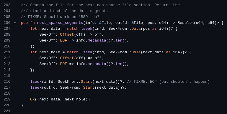
xcp
xcp is a modern partial clone of the Unix cp command in Rust. It is optimised for modern OS filesystems and hardware, and allows experimental features via a pluggable driver architecture, while ensuring reliability by utilising best-practises in functional testing.
Check it out